Introduction

A Bayesian hierarchical model, is a statistical model that incorporates multiple levels of variability or hierarchy in its structure. It is particularly useful when dealing with complex data that exhibits nested structures or when there is a need to model variability at different levels of aggregation. For instance, in forecasting demand for products in a retail chain, a hierarchical Bayesian model may include hierarchical components at multiple levels, such as product-level trends, store-level seasonality, and regional-level effects. By accounting for the hierarchical nature of the data, the model can improve the accuracy of demand forecasts and capture variability across different levels of aggregation.

General idea of Bayesian Hierarchial Model

The mathematics behind hierarchical Bayesian models involves specifying the hierarchical structure of the model, defining the likelihood function, specifying prior distributions for the parameters, and then applying Bayesian inference to estimate the posterior distribution of the parameters given the data. Here’s a general overview of the mathematical formulation of hierarchical Bayesian models:

1. Hierarchical Structure: Hierarchical models consist of multiple levels of parameters that are organized hierarchically. For example, in a simple two-level hierarchical model, there are parameters at the individual level (lower level) and parameters at the group level (higher level). The parameters at the group level are often treated as random variables drawn from a distribution, with the parameters at the individual level conditioned on the group-level parameters.

2. Likelihood Function: The likelihood function represents the probability of observing the data given the parameters of the model. It specifies the conditional distribution of the data given the model parameters. In hierarchical models, the likelihood function typically involves nested conditional distributions that capture dependencies across different levels of the hierarchy.

3. Prior Distributions: Prior distributions are specified for the parameters of the model at each level of the hierarchy. These priors represent the beliefs or knowledge about the parameters before observing the data. The choice of prior distributions can have a significant impact on the posterior inference and should reflect any available information about the parameters.

4. Bayesian Inference: Bayesian inference involves updating the prior beliefs about the parameters using the observed data to obtain the posterior distribution of the parameters. This is done using Bayes’ theorem, which states that the posterior distribution is proportional to the product of the likelihood function and the prior distribution. Mathematically, this can be expressed as:P(θ∣y)= P(y∣θ)×P(θ)/P(y)

5. Posterior Inference: Once the posterior distribution is obtained, various summary statistics, point estimates, or credible intervals can be computed to characterize the uncertainty and make predictions. These may include posterior means, medians, modes, or quantiles of the parameters.

6. Computational Methods: In practice, exact Bayesian inference may be computationally challenging, especially for complex hierarchical models with high-dimensional parameter spaces. Markov chain Monte Carlo (MCMC) methods, such as Gibbs sampling or Metropolis-Hastings algorithms, and variational inference techniques are commonly used to approximate the posterior distribution and obtain samples from it.

A two level Bayesian Hierarchial Model

Given observed data x, the likelihood depends on two parameter vectors \(\theta\) and \(\phi\).

\[P(x| \theta,\phi)\]

and the prior will be:

\[P(\theta, \phi) = P(\theta | \phi) P(\phi)\]

In Bayesian hierarchical models, we typically deal with multiple levels of parameters that capture different sources of variability in the data. To simplify, let’s assume we are working with two levels:

1. Individual Level Parameters \((\theta)\): Parameters that describe the distribution of data points within each group.
2. Group Level Parameters \((\phi)\): Parameters that describe the distribution of the individual-level parameters across different groups.

Example: Student Test Scores

Problem Setup:

We have test scores for students from several different schools.

We want to understand the overall distribution of test scores while accounting for the variability both within and between schools.

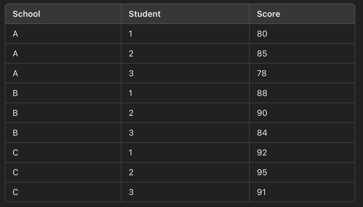
Data: Let’s assume we have the following test scores for students from three different schools:

Level 1 (Student Level): Each student’s test score is assumed to come from a normal distribution centered around the mean test score for their school.

\[y_{ij} \sim \mathcal{N} (\mu _{j},\sigma^{2}_{j})\]

Level 2 (School Level): The mean test score for each school is assumed to come from a normal distribution centered around an overall mean test score across all schools. The school-specific means \(\mu_{j}\) and \(\sigma^{2}\) are being modelled as drawn from higher level distributions.

\[\mu_{j} \sim \mathcal{N}(\mu_{overall},\tau^{2})\] \[\sigma_{j}^{2} \sim Inverse-Gamma(\alpha,\beta)\]

Here \(\mu_{overall}\) is the overall mean scroes across all schools, \(\tau\) is the variance of the class means, and \(\alpha\) and \(\beta\) are the parameters of the Inverse-Gamma distribution governing the school variances.

Now let’s dive a bit more into the mathematics and estimate the scores. Specify Priors: First, specify the priors for the parameters in the model:

• \[\mu_{overall} \sim \mathcal{N}(\mu_{0},\tau^{2}_{0})\]
• \[\tau^{2} \sim Inverse-Gamma(\alpha_{0},\beta_{0})\]
• \(\alpha\) and \(\beta\) hyperparameters for the Inverse-Gamma distribution governing \(\sigma_{j}^{2}\)

Specifying the likelhood: The likelihood for the student scores given the parameters is:

\[P(y | \{\mu_{j}\},\{\sigma_{j}^{2}\}) = \prod_{j}\prod_{i} \mathcal{N}(y_{ij} | \mu _{j},\sigma^{2}_{j})\]

The likelihood for the school-specific means and variances is:

\[P(\{\mu_{j}\} | \mu_{overall},\tau^2) = \prod_{j} \mathcal{N}(\mu_{j} | \mu _{overall},\tau^{2})\] \[P(\{\sigma_{j}^2\}| \alpha,\beta) = \prod_{j}Inverse-Gamma (\sigma_{j}^{2} | \alpha, \beta)\]

Posterior Distribution:

\[P(\{ \mu_{j}\},\{\sigma_{j}^{2} \},\mu_{overall},\tau^2|y) \propto P(y | \{\mu_{j}\},\{\sigma_{j}^{2}\}) P(\{\mu_{j}\} | \mu_{overall},\tau^2) P(\{\sigma_{j}^2\}| \alpha,\beta) P(\mu_{overall}) P(\tau^{2})\]